Category: Volatility
Jul 02, 2014
in Volatility
When you study finance, you have to first learn the basic fundamentals of portfolio theory. When you eventually move to real life, you quickly realize how theory is only a starting point. Nevertheless, it is useful to know the "book theory" because it provides something of a very basic framework. That said, in the words of the great investor Mike Tyson "Everyone has a plan 'till they get punched in the mouth." First, here is the look of a list of ETFs that climb up the risk curve.
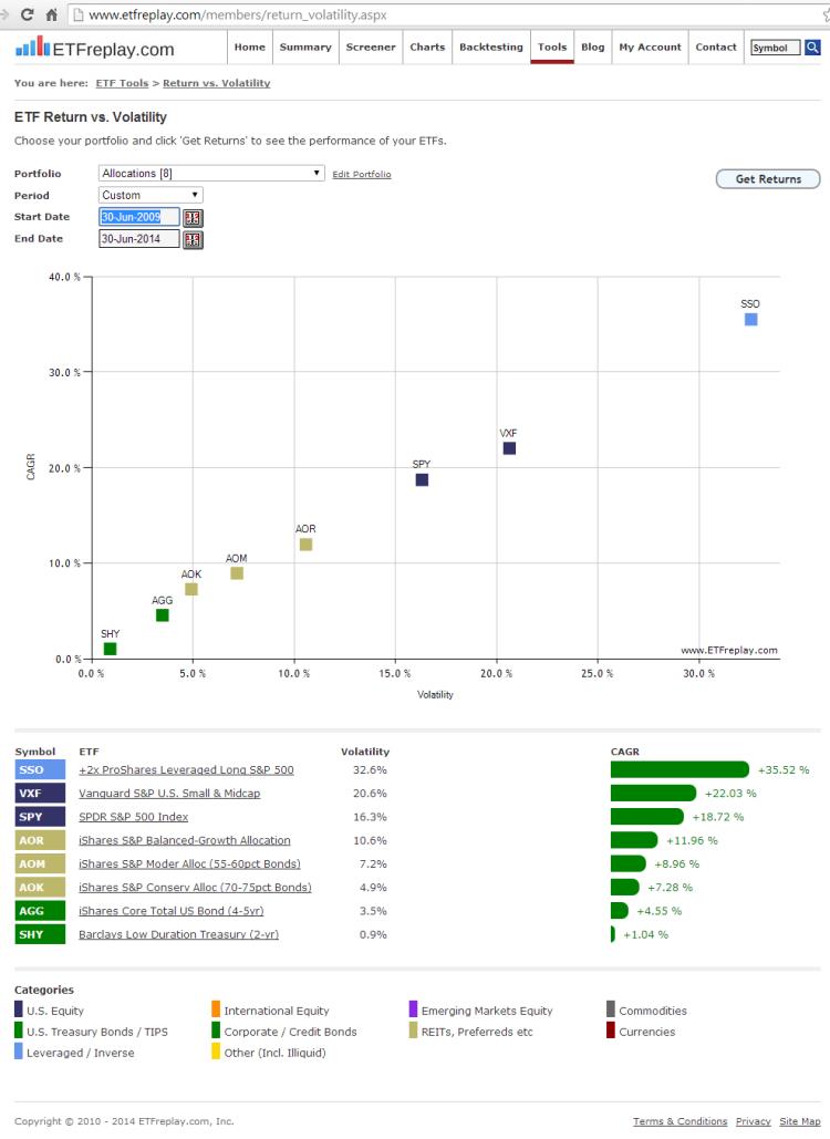
Note that this was posted on this given date covering this very specific time period. Using those precise assumptions, the book theory held up nearly perfectly -- a line going from lower left to upper right --- more return for more risk. But you have to remember --- that was using some very careful selections. Here is an example of a different time period where equity investors were punched in the mouth, Tyson-style:
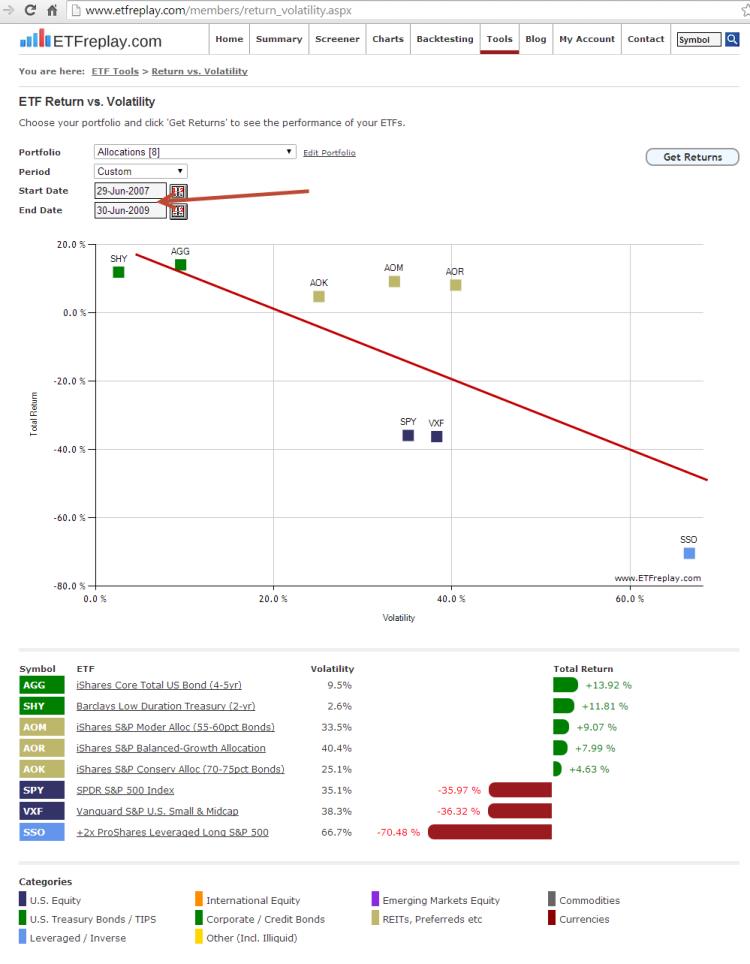
The point is that the volatile ETFs that are towards the right side of the chart will be the ones to have large intermediate-term drawdowns and large intermediate-term returns. The ETFs on the left side will have low drawdowns and low returns. These are very generic ETFs. Where this gets much more interesting is when you use other ETFs that track more interesting indices.
Watch our backtesting videos.
Oct 15, 2012
in Volatility
Risk-parity is a weighting methodology. Given a set of securities in a portfolio, risk-parity overweights lower-than-average volatility securities and underweights higher-than-average volatility securities.
Q. How does it work?
One of the most commonly accepted ways is to start with equal-weight positions and then make adjustments based on the relative volatilities.
Because volatility always embeds a specific time-period assumption, you must specify the time-period (or lookback) you want to use. There is no universal definition on what time-period is correct.
If you choose a shorter lookback period, then your portfolio will adjust more quickly to major changes in volatility. If you choose a longer lookback, then you will have less trading and less whipsaw losses when corrections end quickly and recover.
(for what its worth, we have observed that some index providers use 12-months for the lookback time period and then chooose to rebalance quarterly. But keep in mind that given two different analysts using different assumptions, you will get two different results for the same list of securities within a risk-parity portfolio. As noted, there is no single 'answer').
Q. What is the purpose of all of this?
To us, one of the more interesting problems facing investors are questions having to do with how we weight securities that are in totally different asset classes. Some securities mature at par (bonds) and some are perpetual (stocks) --- some represent paper securities with high yields (preferred stocks) and some can be physical securities that have zero yield (Gold). So long as something is actively traded on an exchange with accurate TOTAL RETURN pricing, risk-parity principles can offer an idea on a weighting methodology that uses the same metric across all of these disparate secruities.
Q. Does risk-parity give an optimal weight?
No. There is no way to calculate an optimal weight for the forward period so risk-parity looks at recent experience and applies that to the future period.
Problem -- if short or intermediate bonds are used, the risk-parity methodology will always very heavily weight bonds (especially lower duration bonds). This is because bonds that have fixed maturity dates will (nearly) always be far less volatile than securities that are perpetual (like stocks). Clearly, low-duration bonds don't have much return potential either so if you were to follow risk-parity, you would end up heavily overweighting bonds relative to something like a 60-40 mix.
Q. Is risk-parity better understood as a concept or as a formula?
While risk-parity sounds quite pleasing, our opinion is that like just about everything in investing, understanding the concept behind it is more important than solving a formula. This goes back to the very basics of investing: given similar return expectations you should choose to more heavily weight the lower-volatility security. This does NOT mean that high-volatility securities are not investable -- it just means that you must have higher return expectations for the high-volatile assets. If your return expectations are indeed higher, then it will make sense to overweight the higher-volatile asset.
Risk-parity will tend to do very well in any period with significant bear markets for an obvious reason, its focus on bonds. Risk-parity will generally (but not always) underperform in up markets for the same reason.
In our view, the point of backtests -- including risk-parity backtesting -- should not be to determine a formulaic 'answer' --- the point is to let backtesting help you digest large amounts of data and be part of the research process that helps you come to a conclusion about what is the right portfolio - in that situation - for that client - at that time.
There are many ways to use volatility to help think about your portfolio exposures and it takes judgment at the end of the day. Given that risk-parity does nothing to adjust for differing return expectations across securities, it should be viewed as simply another tool, not an entire strategy in itself.
-----------------------
Example:
To understand the risk-parity calculation, it is important to realize how a risk-parity portfolio differs from an equal-weight version of a portfolio with the same holdings.
This example will use ETFs from 2 different asset classes: Gold (GLD) and Real Estate Investment Trusts (REITs). Think of it as a way you might want to research how to weight your 'alternatives' allocation. For round numbers, assume alternatives make up 10% of your total portfolio and you want to research how risk-parity handled the past 7 years.
Below would be the weight of GLD using 3-month risk-parity for the period:
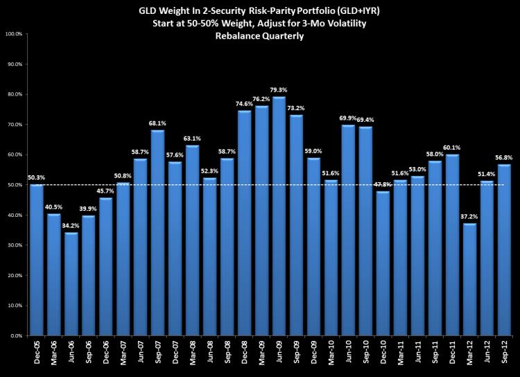
Note that in 2006, the risk-parity methodology had Gold as an underweight vs real estate. At the time, real estate was in the tail-end of a major bull market. As 2007 began, the weightings equalized (signalling equal volatility) and then REITs went into a major bear market and Gold came to be about 75% of the mix for about a year. Since the end of 2010, the weightings have been on average near equal. Note also that over that same time, the returns of REITs and Gold have been about the same.
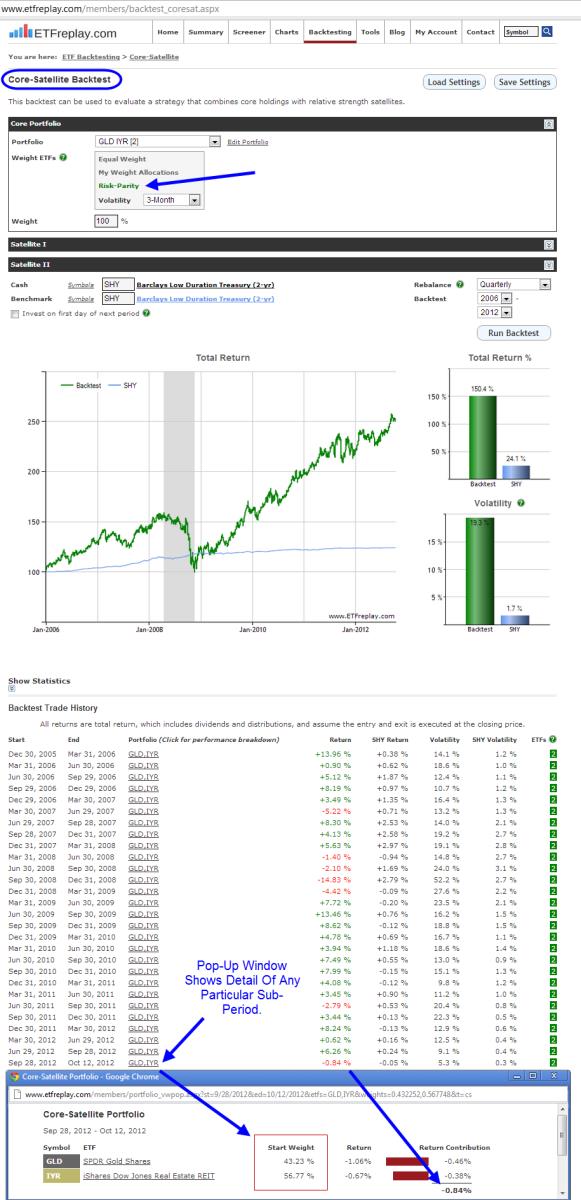
The risk-parity module is embedded within the core-satellite application. Here is a screenshot:
May 30, 2012
in Volatility
A new book in the Market Wizards series by author Jack Schwager has come out this month. While these books are a collection of interviews of great money managers -- Schwager himself also does a nice job of summarizing some of the themes he personally has gleaned by incorporating his decades of experience into a series of observations.
He also recently summarized a few of these observations on his twitter account (@jackschwager)
A few of his takeaways from interviewing top money managers:
- It is not about predicting what will happen -- but rather recognizing what is happening
- Many go wrong by failing to adjust exposures to changing market volatility
This all conveniently ties into ETFreplay, using Relative Strength to help recognize what is happening is foremost. But on the second point, we recently added a module to help think about how to adjust exposures to changing market volatility. Let's look at one example of the latter.
Let's think about the Russell 2000 Index, the most popular index for small cap U.S. stocks, which is one of many important market segments we can access at ultra low-cost (never any redemption fees or lock-ups with ETFs) and it of course has total transparency and is deeply liquid.
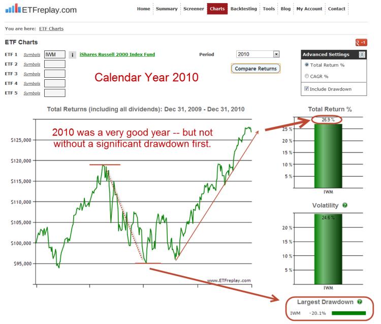
Let's look back at 2010 for an interesting example of how this segment has traded.
2010 was a very good year -- but you wouldn't have said that during the summer of 2010 when there was a large drawdown following a flash crash in May and yes, continual negative newsflow from... drumroll... Europe. The final IWM return was very strong +27% but masks the mid-year washout and pain many investors felt.
Here is 2010 as full year snapshot.
Go forward one year to 2011, the IWM final return of -4% for IWM also greatly masks the 'path-taken.' Another large drawdown, this time -29% and about the same actually as the European index loss (VGK was off -30% from peak to trough).
This is very important and something that investors must study a great deal --- the long-term return of the markets is not all that great in relation to the often wild path taken to get that return. That is, a long-term return of say +7% might have huge drawdowns along the way that cause investors to actually end up losing money if they don't learn how to deal with this.
(In modern portfolio theory terms, you describe this situation (low return relative to high volatility) by saying simply that the Sharpe Ratio is not very good.)
If the short-term S&P 500 sharpe ratio gets really high, just wait -- it's coming back in at some point. This is what happened in Q1 2012 when the S&P 500 YTD sharpe ratio was over 3.00 at one point. We noted this as an unsustainable figure on our Allocations board timeline. And now we see the inevitable washout that occurs with assets that don't have good long-term sharpe ratios. If you want a more efficient equity curve, then don't buy and hold stocks --- unless its part of a well thought-out allocation that adjusts to prevailing conditions.
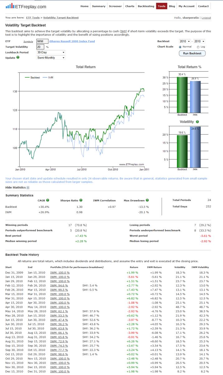
On the ETF Tools page is a new module 'Volatility Target Test.' This module executes a convenient, clean performance backtesting report for you complete with detailed period-by-period weightings and return.
It combines any ETF of your choosing (such as IWM) with a cash-like ETF (SHY) and allows you to therefore approximate a level of volatility for the combination based on changing (dynamic) market conditions. It continually adapts to the current environment and records the performance of such a mechanical targeting approach.
It should be clear that if you target low volatility and the market goes up a lot -- then obviously it will underperform. But if you target lower volatility and the market goes down a lot, it will obviously then outperform. The point of the application is not to be an optimal weighting, it is to help us all understand how volatility targeting is working and how to avoid one of Schwagers main points repeated here
* Many go wrong by failing to adjust exposures to changing market volatility
Below is a single view screenshot of the new Volatility Target Backtest:
Mar 22, 2012
in Volatility
A member wrote a question which spurred some thinking. Essentially, they wanted to understand not just the calculation of the sharpe ratio -- but why its a good metric. So this blog starts on that topic and hopefully can serve as a reference -- it then extends into a longer piece which are thoughts that should help a few people that want to pursue this angle in general.
We are of the belief that you do not want to get bogged down in too much detail beyond this type of math below -- understanding the basic math can be very helpful in your ability to understand investing -- just as understanding the game of Bridge or Poker might be better if you have a basic understanding of the math associated with a deck of cards (total number of cards, number in each suit and how this translates to some basic understanding of odds).
---------------
First -- let us state that the Sharpe Ratio is not a perfect measure by any means (hint: there are no perfect measures) --- but it is a useful framework to start with because it factors in volatility well. High volatility is best associated with large drawdowns, a major concept to keep in mind. What do funds with huge losses all have in common? They were all very volatile.
Drawdowns are obviously your enemy. Trust though that you CAN control your drawdowns somewhat by controlling your volatility. Sometimes you hear how investors want to pair their trades with short-selling. Few investors actually do well with this structure, especially when they pay a big fee. Yes, it's important to hedge your volatility --- but no, you do not need to pay a big fee to a short-selling fund just to reduce your volatility. You can reduce volatility anytime you want and as much as you want and the cost is (should be) very, very low -- they are called short-term bonds. (It goes beyond this post but you can do quite well by using some basic short-term credit strategies -- and then pair these with your core equity/risk strategies that are designed to deliver long-term return).
You DO need to take on some volatility in order to generate some return -- but nobody who actually knows what they are doing is going to be impressed with making X% if you do it with massive drawdowns.
So let's look at some basic math:
1) Compounding returns:
Let's start at some very basics, skip this and go to #2 volatility if you so desire.
Let's start with a 10% annual return. To convert 10% to a daily return, you only need to know how many days there are in a year. Most traders will know that there are 252 equity trading days in most years (fixed-income and foreign markets like China have far fewer trading days due to extra holidays but this actually doesn't matter because the ETFs are open for trading on exchanges even when the underlying market is closed).
So to take 10% down to a daily level in a spreadsheet: place 0.10 in cell A2 and then in B2 type =(1+A2)^(1/252)-1. Now you have a daily figure of approximately 0.0378%. Then practice by reversing it back to the annual 10%. It may be easiest like this =((1+.0378)^252)-1 = 10.000%.
How is this equation useful? Well, for each $100,000 in your account, a 10% annual return would be about the equivalent of 40 bucks a day (lower in the early days and higher in the later days due to compounding for an average just under $40). $40 doesn't seem like much does it? A lousy ~$40 on my $100,000? Yes, that is what 10% a year feels like from a daily compounding perspective (40x250= $10,000).
Let's move to a monthly figure as we find this to be a very useful timeframe, you will see why when we discuss volatility. 252 trading days in a year means 252 / 12 months = 21 days per month, on average. Let's take 10% and convert to a 1 month (21-day) figure =((1+.10)^(1/12))-1 = 0.797% per month.
Just to do the math a different way, let's go from daily to monthly (from above) = (1+0.0378)^21 = ~0.797% per month.
So that is return basics, now let's look at volatility. If you can just get these 2 items (return and volatility math), you will have the 2 major Sharpe Ratio components:
2) Volatility is a slightly different animal but isn't as hard to think about as you suspect. If something goes up a little bit ON AVERAGE each day (like the stock market) but not steadily compounding as in example above, then there is a different dynamic to understand.
Volatility grows not at time -- but at the square root of time. It sounds scary but its not. All that means is that even though the market moves around a lot on a day to day basis, if you look at it over a longer time period, much of those days offset each other and so you can't compound volatility like before because volatility relates to the path taken rather than just the final return result. Think of it as more 3-dimensional analysis. It's trickier -- but it's very important information.
Whenever you take the square root of a number greater than 1, the number is going to get smaller so =sqrt(12) is obviously a lot smaller than 12. This reduction is taking into account the fact that up and down days (volatility) offset each other to a significant extent. So up +10%, down -10%, down -10%, down -10%, up +30% is an awful lot of movement but only gets you back a little positive. The final return of +4.2% doesn't tell you about the path taken.
So if we look at the S&P 500, we can say something like -- over the past X years, the annual volatility has been about [16%] (brackets just mean fill in whatever number you would like, this is just an example).
Volatility is always discussed as an annualized amount. But we can of course convert 16% to a daily figure using an equation like this =(0.16)/sqrt(252) = ~1%.
So given a forecast of 16% volatility, we would now not be at all surprised to see the market go up or down +/-1% tomorrow. There are of course many other possibilities --- but we would not 'expect' it to move 5% --- because if it did, that would be too far from our baseline range of expectations. Yes, it could happen but then that would be associated with rising volatility far above the example 16% used -- our 'forecast' of 16% was wrong in that case. Remember, we are just trying to understand the mechanics of the Sharpe Ratio, we are not trying to forecast 1-day movement.
Now, what practical use does this all have? Well for one, don't try to pinpoint exactly why the market went up or down 1%, it's not a significant enough move when you are looking at it in the context of a few months. Yes, there may be some headline news that day -- but many times the market will do the exact opposite of the nature of the morning headline. It's just short-term volatility in play and it's normal.
We think it makes a lot of sense to look beyond daily movement and toward longer windows of time -- but not too long. A lot of modules on the website are set-up with this in mind. We need a time-period that allows some of that offsetting volatility to work itself out. There is no single magic time-period but various academic papers that we've been reading for the last 15 years point to 1 to 12 months as a good time-period to study. Shorter than 1 month is too noisy and at 12 months or longer, the edge evaporates.
So let's take an example. Let's assume a 2% 1-month return and 16% ANNUAL volatility estimate.
First annualize the return: =((1+.02)^12)-1 = 26.8%. A quick comparison of 26.8% to 16% = 1.68, that is a measure of return divided by a measure of risk. You are risk-adjusting the return into a pretty straightforward ratio. That is, you are incrementally penalizing the return if it took a wild path to get there. If that makes sense to you on a conceptual level then you are 95% of the way there.
You should quickly see that 26.8% is an unsustainably high number. You may have a great year where you do far better than 26.8% --- but you won't be able to compound at this number for the long-term. So here is the logic, since 26.8% annual is unsustainable -- that means 2% a month is unsustainable (it's the same number). And while you may have many months far better than +2%, in order to get a good return/risk situation, you are going to have to also spend a little time thinking about the volatility -- you won't be able to do a good sharpe ratio based on return alone (over the long-run). And of course, the real reason to control volatility is so that you don't experience large drawdowns.
Now let's look at a leveraged fund as that is an interesting phenomenon to think about. A leveraged fund is DESIGNED to have 2x or 3x the daily return of the unlevered fund. The funds will re-balance daily (if necessary) to achieve the next days targeted change. As you should be able to see from above, we know it's a bad idea to trade off 1-day movement because historically (and consistent with the concept of volatility), the market doesn't go up at its long-term rate, it goes up and down in offsetting nature and then only over a larger sample period can we see a return figure that is not so highly skewed.
What this means is that leveraged funds rebalancing daily is a serious long-term flaw and should not ever be held for significant periods of time. This by the way is exactly what the trading in these funds indicates as most of the leveraged funds have low assets relative to their high daily volume amounts. There is much trading during the day and then a lot of people flee before the close.
Back to the Sharpe Ratio. The ideas in this blog have gone into some math but should be thought about more conceptually in our opinion. So to speak from these basic concepts, you could put this into a practical statement in a few different ways (just by re-arranging the key factors):
1. We target a return of 10% a year. We target volatility just below that. (This implies on a conceptual level a reward-risk ratio of 1.0 or better).
2. Volatility has been about 10%, we think we should be able to do a sharpe ratio of 1.0 so that means we think we will do 10% in return or better.
3. We target a sharpe ratio of 1 or better -- we are tactical so volatility will fluctuate up and down -- we aren't going to micro-manage it but we can say that we will manage volatility such that it is no higher than the [S&P 500] index volatility. This means/implies that our drawdowns should always be lower, too.
etc...
Now, let's pretend you were rotating between 3x leveraged funds. How would you rationalize this if in a client meeting??
"Our funds volatility has been running 45% so hey, if we can just do a 0.5 sharpe ratio -- then expect us to compound at 22.5% per year"
Uhh no, the meeting would end there and you would be laughed out of the room. Again, you can and should have some big individual years that put up some nice performance numbers if you execute your strategy well. But we aren't talking about that, we are talking about long-term compounding.
Lastly, let's make sure we end on some common sense. Don't get too mathematical about all this. At the end of the day, this is about growing your account balance. Making new all-time highs in your account balance and not having large drawdowns is efficient money management. If you do that, who really cares whether you did X% or X+1%? Don't lose sight of the big picture by getting too bogged down in the exact math. An understanding of the concepts is needed -- an exact knowledge of every nuance in the calculations is not.
Dec 22, 2011
in Drawdown, Volatility
We are updating our 'Volatility vs Subsequent Drawdown' Chart for 2011. We did a similar post a year ago and you can review that blog post here: Understanding ETF Volatility Part 1.
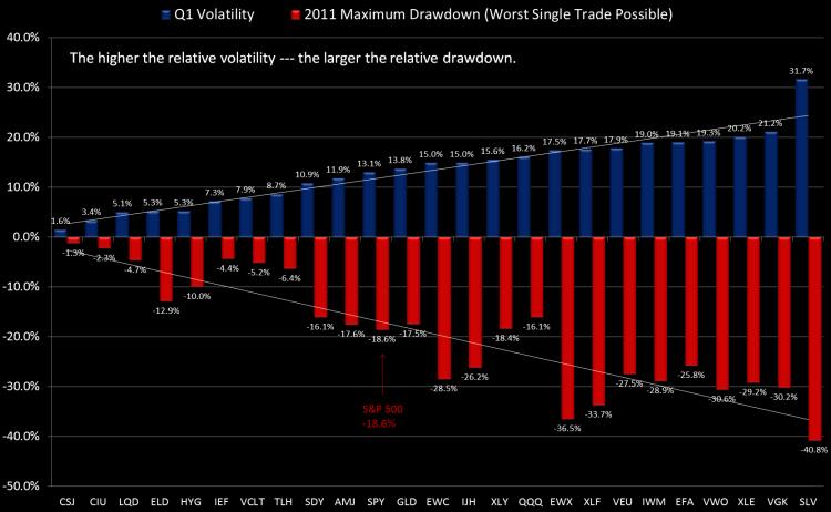
The way to read these charts is to simply note the relationship. By definition, high standard deviation investments offer wider opportunities for both out and underperformance. The S&P 500 dropped -18.6% off its high during 2011 (using closing total return values). This was -3.2% worse than the mid-year loss in 2010, when the S&P dropped -15.6%.
Gold had a more normal drawdown in 2011 at -17.5% vs 2010's -7.8%, due mostly to its more aggressive slope up during the summer. Gold never got particularly volatile in 2010 but in 2011 it traded more typical of a commodity market -- where there is often a momentum-oriented blow-off move. Still, if you were watching volatility dynamically, you would take note of it becoming riskier during the July-August advance.
The NASDAQ-100 actually dropped slightly less from high to low in 2011 vs 2010. Large-cap tech -- particulary AAPL have been relatively calm in 2011 -- which was also the case in 2010. Can it go 3 years with just a mid-teens drawdown? We don't know but there are certainly other more attractive segments as we close 2011.
It may sound odd but the losses in both 1) small cap US stocks (IWM) and 2) US Energy stocks (XLE) were about the same from high to low as the European ETF (VGK), which dropped -30%. However, both of the US ETFs have seen strong rebounds in Q4 and are a few percentage points from flat on the year.
Silver (SLV) is pretty consistently the most volatile (unlevered) ETF around and it didn't disappoint with a -41% high to low move in 2011 (and the year isn't quite over).
Treasury bonds ground out fantatstic years. We've blogged many times about how intermediate and low-duration bonds are the ultimate safe-haven. You can't count on consistent correlations in times of crisis -- but you can count on low-duration bonds, the fixed-maturity dates of the underlying securities ensure it. This is not true of long-term bonds -- which look susceptible to significant drawdowns in 2012. As much hype as the US downgrade received, it proved yet another meaningless move by the ratings agencies in the United States, which for some antiquated reasons seem to remain relevant to some.
Note that many ETF providers launched 'minimum volatility' ETFs in 2011. Since starting ETFreplay.com in early 2010 we have always used volatility as 1 of 3 key inputs in our multi-factor screener model -- so we are not surprised to see this development from the ETF providers. Volatility has and always will be important --- but it's certainly not the only thing that matters. Myopically focusing on volatility is taking this all too far as building ETFs off a singular concept like this is very limiting.
We view risk-adjusted (volatility-adjusted) relative strength as the cornerstone philosophy of ETFeplay.com and this led to a fixed-income bias throughout most of 2011. However, a tactical investment process continually looks to adapt to the environment --- and we would look for continue rotations in 2012 --- and every other year for that matter. There is plenty of room to add value in any year and it's up to you to figure out which group that is and how to manage it. In 2011, fixed-income ETF showed excellent total returns. You can't always be right of course --- but you can pursue a process on thoughtful consideration of which markets to be involved with --- and then layering some trend-following techniques on top of that --- all the while continually striving to protect yourself for the times you are wrong. If you simply stay consistently loaded in a group of highly volatile securities -- it is just a matter of time before you have a large drawdown.
As can be seen in our tracked Portfolio Allocations, we view equities to be attractive as we end 2011 -- particularly small and midcap US stocks. We see signs of P/E multiple expansion with rates low and liquidity being added to the problem areas of the global economy. However, even assuming we enter an intermediate uptrend (which may or may not occur), this does not mean that more rotations within the markets won't occur. It is never easy in the moment and we will carefully continue to watch and adapt to new potential themes/trends --- while always watching our backs to avoid too much portfolio volatility (and its associated drawdown).